Index Match: The Better Alternative to Vlookup

VLOOKUP is one of those functions that make Excel great. Although many may not find it intuitive at first, it soon becomes second nature and indispensable. Some even find is life-changing. VLOOKUP has its issues though, for one, it only reads from left to right. If you need to look up a value to the left of a reference column, you’ll have to rearrange your worksheet to use the function.
VLOOKUP also canvases many columns when in actuality you are only using two of them. the standard syntax only references relative column values, if you modify the table you are out of luck once again and need to do a little bit of reorganizing and function rewriting, which can be very tedious in large workbooks. This also creates issues in copying the function to other columns.
There is an alternative though, INDEX + MATCH. Not only does it replicate the functionality but has its own perks and bonuses. It’s something you may not have heard before (especially if you don’t read about Excel for fun) but by the end of this article, you’ll be able to put it into practice and reap the rewards.
Breaking Down INDEX + MATCH
Something that many users overlook is that Excel functions can be chained together and combined to make something even more powerful than the constituent parts. Each function takes an argument, if you need a little more power or extended functionality, these arguments can be made of other functions.
INDEX
=INDEX(array, row number)
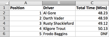
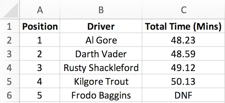
The INDEX function takes a user array, a set of values such as a column, and returns the value of the cell at that particular position. For example, I have a column of data recording the positions from a race held at some point in the past. I want to know which driver finished in third place, to find this I can simply enter,
=INDEX(B2:B6, 3)

and this will return Rusty Shackleford.
Simple but useful. We now have the ability to return values within an array.
MATCH
=MATCH(lookup value, lookup array, match type)
MATCH() is another simple function, related to the INDEX function we just covered. Instead of returning a value though, it instead returns a number signifying the relative position of a value within an array. MATCH requires the following arguments; the value, the array to search, and the match type. The match type will usually be set to 0 but depends on your usage. 0 signifies you only want an exact match, 1 or -1 signifies if there is no exact match you want the next closest value.
Using our race example above, I know the driver I need to find but I don’t know his position in the final race standings. Since the position is relative I need to make sure I cover the entire results starting from the first position.
=MATCH(“Kilgore Trout”, B2:B6, 0)

This will return a value of 4. Since we started from the top we know Trout finished in the fourth position in this particular race.
INDEX MATCH
Maybe you see where we are headed now or maybe you skipped ahead to get to the good stuff. Using INDEX + MATCH we can combine these two simple functions to make something similar but more flexible than our trusty VLOOKUP. Don’t worry if you need to read through this a few times, it can be a little tricky at first. Once you grasp what is going on though it’s really easy to rebuild it from the components.
INDEX returns a specific value. This is the primary function of VLOOKUP, given a set of parameters; you can quickly find a needed value. Now the only thing we are missing is a way to find the row position. If you have to find this manually you lose the utility of a function. By using MATCH in the second argument we can take its output, a relative position, and push that into the Index function, solving that problem. Now we have something that does the exact same thing as VLOOKUP, with only a little bit more typing.
Putting the Function Into Practice
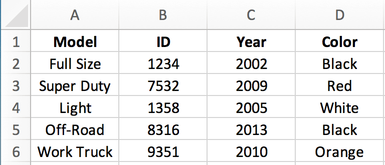
Using the table below, we are interested in figuring out what product type is associated with a specific product ID.

To use INDEX MATCH we start with INDEX since ultimately we want a specific value returned rather than a position. Inside the INDEX we include MATCH to return a position for our INDEX function.
=INDEX(A2:A6,MATCH(8316,B2:B6,0))
What is happening here is that I am going to search column A for the value of the row in column B, provided by the Match function.
Inside the match function, I specify that I need to look through the Product ID codes in B2:B6, and send back the position of the value 8316. In this case, it is in position 4 which is the equivalent of writing
=INDEX(A2:A6, 4)
Excel runs the function and finds the position in the array of the specified ID number. It takes that position and looks for the same row in our A column, returning the truck type for the specific ID. So, in the end, we get the same results with a little more flexibility in the inputs.
The Function’s Perks
INDEX + MATCH’s power comes from the smaller data selection. If you have 15 columns but you are only using numbers 1 and 15, why pull everything else in? This can help speed up the running time for large data sets.
The second enhanced functionality the that Index can read left or right, no matter where you put the columns, INDEX is indifferent to whether it is to the left or right of your initial array, unlike VLOOKUP. If you look again at the example above, that is just what we did, working from right to left. The function can also serve as a quality assurance check since you must manually specify the two columns you need rather than enter a relative column number somewhere within your selection.
Conclusion
Go ahead and play around with INDEX + MATCH. It’s a very powerful function that can enhance your lookup abilities. Once it clicks, I’m sure you’ll be sold and never look back. There is always a bit of a learning curve when trying something new, commit to using Index Match for a while. It’ll be clunky at first but you’ll art seeing the benefits shortly.
———-
Post updated by Jenna Kelly (prior post date: 2/3/14)


