How To Perform Excel Lookups With Multiple Criteria

Everyone loves Vlookups, the formula that helps us quickly match data across our ever-increasing Excel tables. However, there is a glaring weakness – lookups for multiple criteria. Vlookup accepts one value in its first parameter. Need more? Well, that is too bad as the technology just isn’t there yet so break out your pencil and paper, you’re going to be here a while.
Now that you’ve braced yourself for the impending slog, I’m happy to tell you there is an easier way. Depending on how adventurous you are feeling, you have quite a few options. In this article, we’ll discuss Vlookup examples for the purists and a couple of other functions for those who want to live more wildly.
Simplest Solution: Helper Columns
The simplest solution involves introducing at least two columns to our buddy, concatenation. By combining multiple cells into one value, we can use the concatenated cells as our look up, bypassing the need for any sleights of hand or Excel sorcery.
For example, we have the same ad group name in multiple campaigns. If we look up by ad group we are not guaranteed to find the correct ad group. The lookup will return the first matching ad group it finds. If we need to match the campaign and ad group, we can combine the two and match that value instead.

You can even concatenate with special characters to make it easier to break them down later. With a combination such as “Campaign | Ad Group”, you not only make it more readable but establish a clear indicator for division between criteria. If you need to reverse this, you can use text to columns to break them back down into separate columns.
Simple Solution Sidebar: Skipping The Lookup Entirely
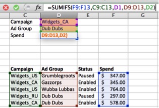
In some cases, you can skip the Vlookup entirely and use SumIfs. SumIfs allows you to sum values based on multiple criteria.
The downside to this method is that SumIfs works with numbers but not with strings. This means you can return numbers (clicks, impressions, cost, etc.) but not strings (status, descriptions, IDs, etc.).

In this case, we use the campaign and ad group column as our criteria and when both match, we sum up the cost. While this isn’t as fancy as the other solutions, it’s extremely convenient.
More Advanced Solution: Index Match With Arrays
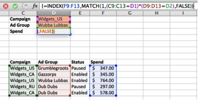
We’ve covered index match before as a more flexible alternative to Vlookup. Combining it with arrays and simple logic turns the functions into a multi-criteria lookup. In essence, we’ll choose our lookup column and the ranges containing our criteria. If all of them evaluate to TRUE we get a match and return the appropriate value.
{=Index(Return_Range(Match(1,(Criteria_Range_1 = Criteria_1) * (Criteria_Range_2 = Criteria_2),FALSE))}

Since this is an array formula you’ll need to execute it with CTRL+Shift+Enter or CMD+Shift+Enter to get the correct results. If it helps, the match segment is translated as check these ranges for a value of 1. Why are we looking for 1? I’ll give you a hint – it’s a logic problem.
We often use TRUE and FALSE as they are equal to 1 and 0 respectively. When we run the match function, it looks through each column for a match. If there is a match it returns 1, if not it returns 0.
Notice the multiplier between the two as anything multiplied by 0 evaluates to 0. As a result, the only time it will return 1 is if we match both criteria and it evaluates as 1*1, which equals 1.
Going All In Solution: Introducing Choose
The first solution included helper columns. This requires inserting additional rows into your spreadsheets. That isn’t a major problem but it can be annoying and require a little extra formatting and clean up. What if you could do all of this without inserting the columns?
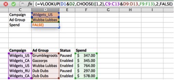
Welcome the Choose function. By utilizing an array function we can create a virtual table for our Vlookup, skipping the need to manipulate the original.
Unlike the last example, we’ll go back to our old pal, Vlookup. In this case, we’ll choose the values we are looking for, set the lookup table, and so on. Only this time the table will be virtual so we’ll build it inside the function!
{=Vlookup(Criteria1&Criteria2,choose{1,2}Criteria1_Range&Critera2_Range,Lookup_Range),2,FALSE)}

Similar to the previous example, the middle is where the magic happens. This explanation requires a bit of reading on your own but the quick version is, the Choose function helps build a virtual table of two ranges. In this example it merges the two criteria into a virtual helper column with the second column being the values we want to return.
Then we continue the Vlookup as normal. Our values are in the second column we set up, so we set it to 2 and it runs just like any other Vlookup.
Conclusion
Some of these formulas will take a bit of practice before you are conformable with them. Most of them have very similar outputs, though, meaning you can choose whichever you prefer. Although we only used two criteria in our examples, all of these formulas can be extended to include more. Play around with the examples in your own workbooks and see what works best for you. You might even stumble across your own solution or style.


