
Every now and then you stumble across an Excel tip or trick that blows your mind. However, this won’t always be the case and as your skills progress these insights are harder and harder to discover or take more effort than they are worth.
Rather than going bigger, it is often much easier to take a step back and recognize little tricks you could try, or actions that lead to fewer errors and easier spreadsheet management. Since we just rolled over into a new year, why not start off 2015 covering a few tricks to amplify your work?
Use Cell References Whenever Possible
Instead of copy and pasting or duplicating your data across the workbook, use cell references in your tables. This strategy not only keeps you from making unintended errors with simple numbers but also gives you a single location to reference the data in the case something looks off. In the event that a table or formula has an error, rather than back tracking your steps through the workbook you can simply check your cell reference to make sure it matches up. In the event that this workbook will sit for a while before being viewed again, making liberal use of references can make it easier to reacquaint yourself with the details of the specific book.
Label Your Pages and Data Consistently
One of the worst things that could happen in a spreadsheet is that everything you’ve done is incomprehensible. To avoid this make heavy use of explanatory labels and accurately title your sheets. There are no set rules for these so you can take as much freedom as you see fit. Nonetheless, I find including the intent of a page to be vital in showing which pages are valuable and for what reason.
As an example, lets pretend I’m creating a year end report on AdWords performance. I may start with the basic ad group report from AdWords and from there I create separate sheets for each. For my formatted ad group data I may title the original sheet, “Raw Data” and the formatted sheet “Table – Ad Group Data”. If I were to amalgamate the ad group data into campaign level data, I would in turn create a “Table – Campaign Data”.
You can further enhance this process by coloring your tabs with a certain pattern. For example you may gray out your data sheets to deemphasize them, or use a single color to highlight sheets regarding revenue data – blue for conversion focused data and so on. Alternatively, depending on the viewer, you may opt to hide the data sheets completely if they add nothing to the workbook.
Even if you only implement small changes, the small perceptual cues will make it easier on the viewer. They may not mention it, but avoiding unnecessary questions is an easy way to increase your effective communication.
Formatting
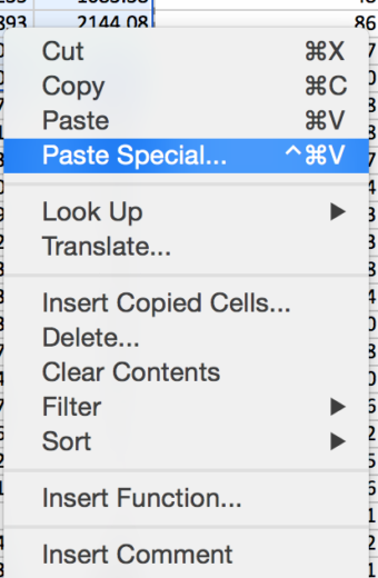
This topic is huge from both a design and usage standpoint. Nonetheless, keep your formatting consistent to improve readability and allow you to use shortcuts like pasting formatting options. For instance you may have a workbook full of individual tables with monetary units, text formatting, percentages, and more. It’s awfully annoying, even with shortcuts, to fix these piece by piece. If you have the same table set up, simply set one up the way you want it and “paste special” format over the rest of them.
Secondly, make use of cell formatting, conditional or otherwise. Personally I hate excluding data and try to include as much as possible in my workbooks. Taking our year end report example what can I do to keep paused entities in the report but also point to the fact that they are no longer running?
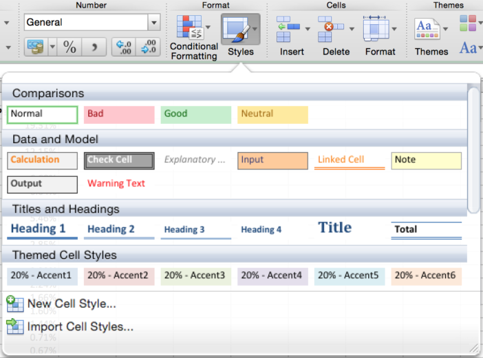
Before you say it, yes there is a column for status but why force the reader to scan the columns or change the filters. In these cases I personally like to use the “explanatory” cell formatting to mute the text with a light gray. It’s still visible but clearly muted in the mix of active entities.
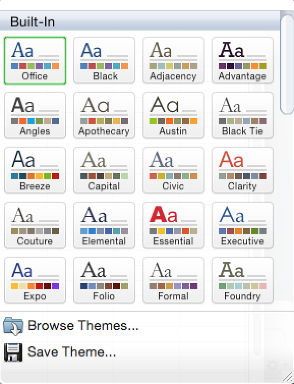
Picking a color scheme isn’t everyone strongpoint. Even if you can, sometimes it’s nice to pass off the task to Excel itself. Excel is loaded with predefined color schemes that you can select and automatically apply to your sheets. One click and your reports look better – why wouldn’t you use it?
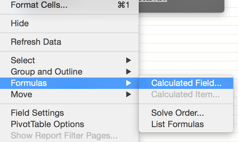
Use Custom Fields in Your Pivot Tables
While the earlier tips were somewhat abstract and conceptual, this final tip may or may not hit you with the blunt force of a public service announcement. Almost everyone is using pivot tables these days but every now and then I still see formulas along the right hand side of said tables.

If you need to include fields like CPA, which may be butchered by the default pivot table options, simply right click inside the table and “insert custom field”. This will open a new menu in which you can mix and match fields and formulas creating the compound metrics you need. Now with the bonus of integrating with your pivot table, allowing you to use it in any configuration of said table.
Conclusion
By revisiting the basics, you’ll often find better ways to do something. Rather than giving you the ability to do something new, these tricks will amplify your future work as your improve your skills from the bottom up.
What are your favorite techniques for managing and presenting your spreadsheets? Even if the tip is super specific to your work there is a seed of an idea in there that could help someone else in their own work. Feel free to share any tips in the comments below, on Twitter, or shout it from the rooftops.
